
The Gugelmann Collection1 consists of roughly 2300 items that are so far digitised. In a first round of this project, three different aspects of information contained in the images or the accompanying meta-data have been analysed. None of them, however, was able to grasp an idea of the subjects and their composition represented in the image.
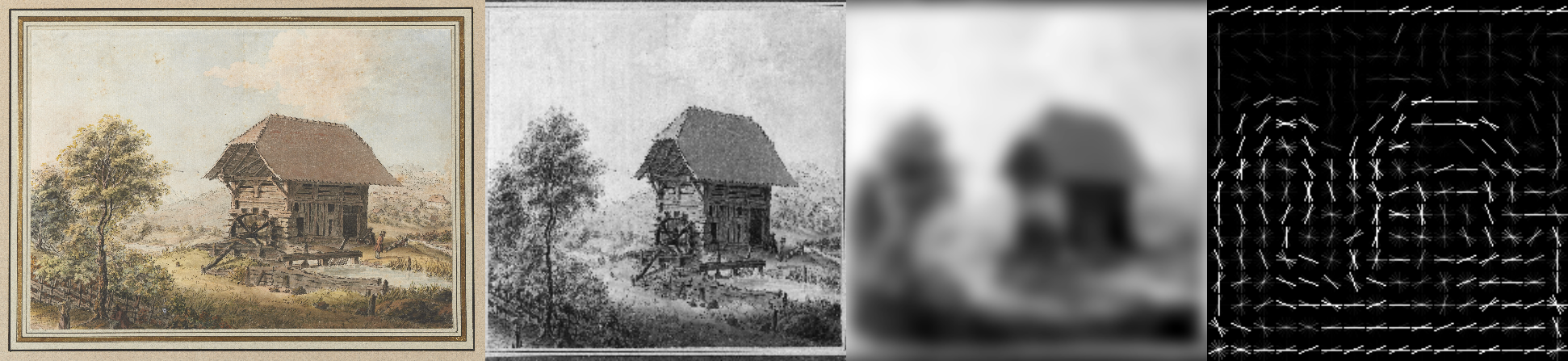
1: original image / 2: scaled, cropped, black and white / 3: Gaussian blur / 4: histogram of oriented gradients (HOG)
In order to be able to compare images among each other with respect to their composition, a series of image processing operations have to be applied to each of the items. First, the original images are converted to grey scale. Then they are cropped to get rid of borders, that would have a unnecessarily high influence on the result. To the downsized version, a Gaussian blur is applied to prevent local details from influencing the overall result. This image is then split into 8∗8 tiles, for each of which the intensity of gradients in 8 different directions is analysed.2 This results in 8 ∗ 8 ∗ 8 = 512 dimensions for each image. A manifold learning algorithm called TSNE3 is then applied to reduce these 512 dimensions to two to allow for a visualisation of these neighbourhood embeddings.
A three dimensional embedding can be virtually explored in the Gugelmann Galaxy. Direct link: http://www.mathiasbernhard.ch/gugelmann/
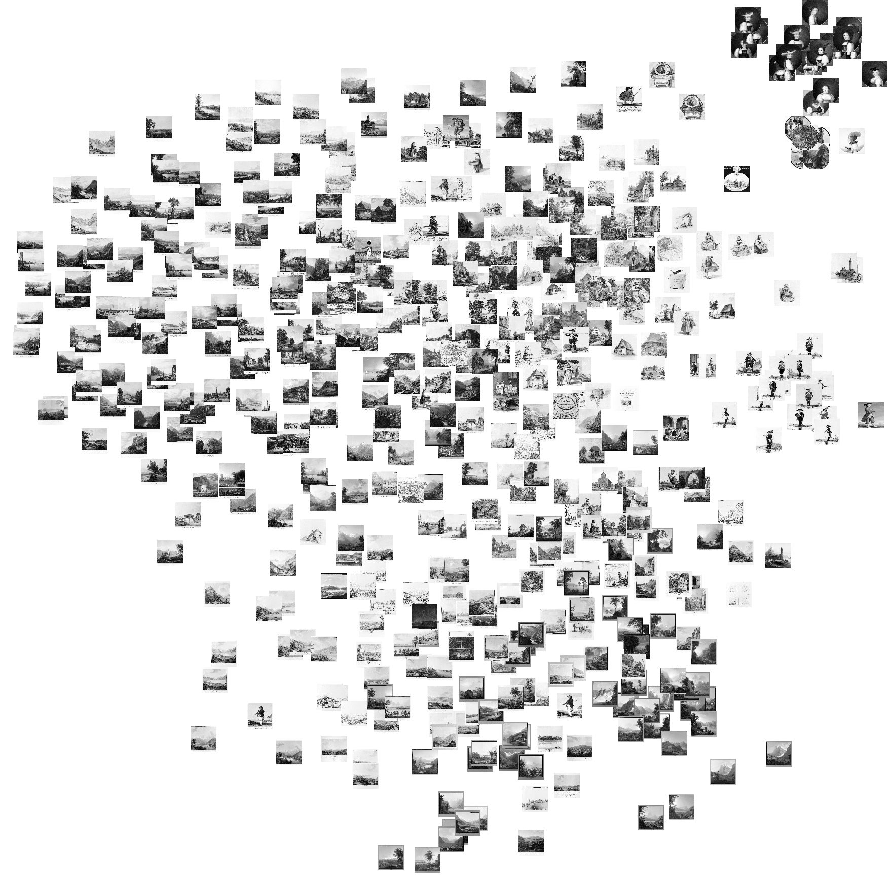
TSNE projection to 2 dimensions for a subset of 500 images
Similar images are close to each other, while big differences force images to separate apart from each other. The above figure shows a subset of 500 images at their respective X-Y-position, calculated by the machine learning algorithm. Since the numerous overlaps impair legibility, the below figure shows the items forced into a grid.4
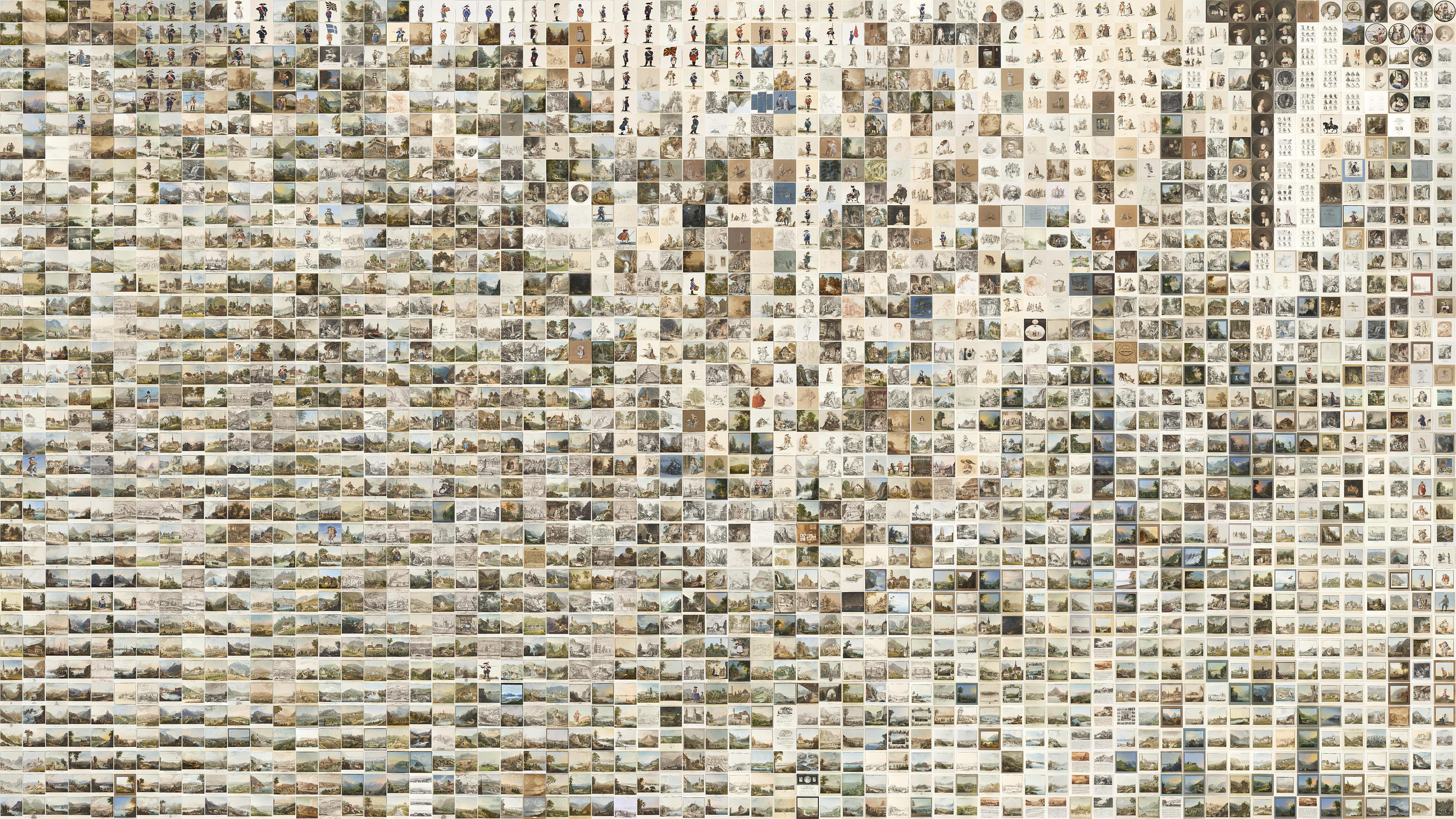
TSNE projection to two dimensions, rearranged into a 64 x 36 grid of square tiles (click to enlarge)
Some compositional concepts become obvious at first sight, such as the circular vignettes in the top right corner, upright figures on a neutral background a bit farer left, wide landscapes in the bottom left or images maintaining a frame despite the cropping in the bottom right. Some of these clusters (landscapes, soldiers on white background or the women portraits in folk costumes) already emerged from the sorting according to color distribution. A notable improvement can be illustrated by a group of images at the bottom, a bit left of the center (see figure below).
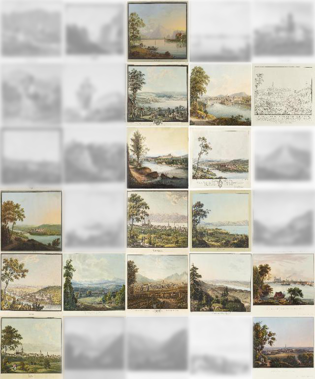 The similarity of of these images’ composition (foreground tree at the left, landscape – often with lake – in the background) could by no means be discovered in the meta data. The images are by different authors and represent different places. Also the color clustering would not arrange them in close proximity because they are very different in sky color and overall tonality. Even a very light pencil sketch (2nd row, right) can be found in this cluster, something that from a computer vision system point of view – that is, dealing uniquely with a matrix of numbers for red, green and blue values – really looks different.
The same procedure of clustering can be conducted with basically any collection of images. Here is the result, applied to a small set of the WikiArt collection. Only works of the genre “cityscape” are taken into account and, for the sake of speed, only a subset of 578 of these images. The visualisation is not only a static image as above, but lets the user hover over items to enlarge them and see meta data like title, author and year. Interesting in the sense of a proof of concept is the group of “Boulevard Montmartre” paintings (by Camille Pissarro) under different weather, time and light conditions at the right border.
http://www.mathiasbernhard.ch/wikiart/
- paintings and drawings by Swiss artists, provided by the Swiss National Library (SNL) as open data
- This procedure is called HOG for histogram of oriented gradients, an algorithm often applied by computer vision systems for object detection.
- t-Distributed Stochastic Neighbor Embedding
- Items are first sorted by their x-coordinate, then in junks of N (number of rows) sorted by y-coordinate. Admittedly not the most elegant way of doing it, but works.